Conduct Semiparametric Latent Class Analysis for Recurrent Event.
Usage
SLCARE(
  alpha = NULL,
  beta = NULL,
  dat,
  K = NULL,
  gamma = 0,
  max_epoches = 500,
  conv_threshold = 0.01,
  boot = NULL
)
Arguments
- alpha
initial values for alpha for estimation procedure. This should be NULL or a numberic matirx. NULL means obtain initial value with k-means.
- beta
initial value for beta for estimation procedure. This should be NULL or a numberic matirx. NULL means obtain initial value with k-means.
- dat
a data frame containing the data in the model
- K
number of latent classes
- gamma
individual frailty. 0 represents the frailty equals 1 and k represents the frailty follows gamma(k,k)
- max_epoches
maximum iteration epoches for estimation procedure
- conv_threshold
converge threshold for estimation procedure
- boot
bootstrap sample size
Value
A list containing the following components:
- alpha
Point estimates for alpha
- beta
Point estimates for beta
- convergeloss
Converge loss in estimation procedure
- PosteriorPrediction
Posterior prediction for observed events for subjects of interest
- EstimatedTau
Posterior probability of latent class membership
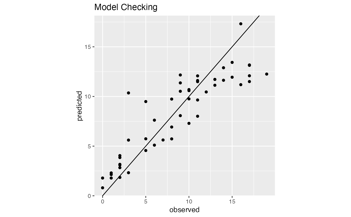
- ModelChecking
Plot for model checking
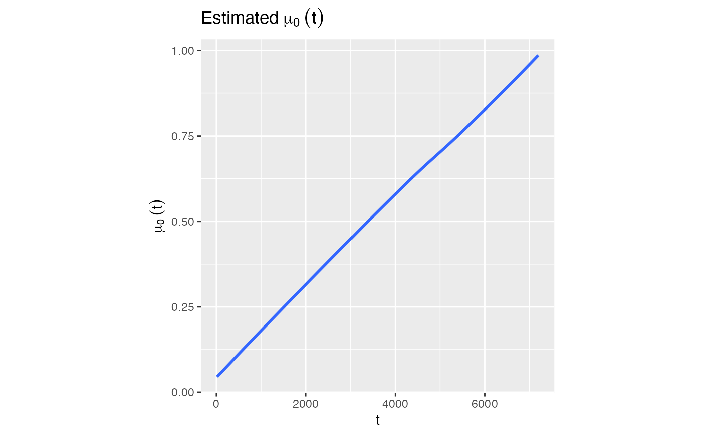
- Estimated_mu0t
Plot for estimated mu0(t)
- est_mu0()
A function allows to calculate mu0(t) for specific time points
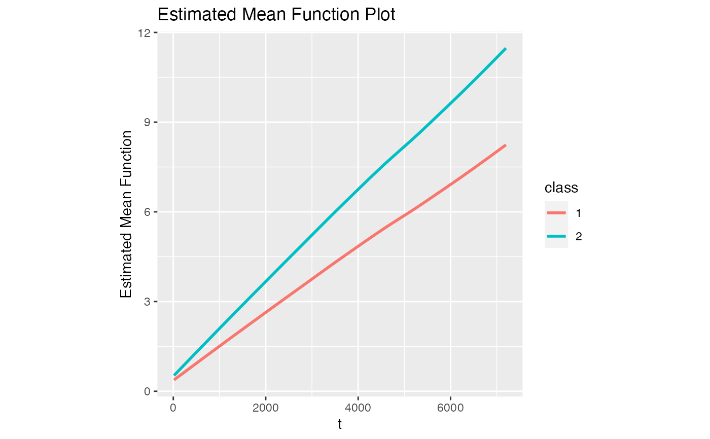
- Estimated_Mean_Function
Plot of estimated mean functions
- RelativeEntropy
Relative entropy
- InitialAlpha
Initial alpha for estimation procedure
- InitialBeta
Initial beta for estimation procedure
If argument 'boot' is non-NULL, then SLCARE returns two additional components:
- alpha_bootse
Bootstrap standard error for alpha
- beta_bootse
Bootstrap standard error for beta
Examples
data(SLCARE_simdat)
# Example 1: number of latent classes k = 2,
# By default, generate initial values in estimation procedure with K-means
model1 <- SLCARE(dat = SLCARE_simdat, K=2)
# contents of output
names(model1)
#> [1] "alpha" "beta"
#> [3] "convergeloss" "PosteriorPrediction"
#> [5] "EstimatedTau" "ModelChecking"
#> [7] "est_mu0" "Estimated_mu0t"
#> [9] "Estimated_Mean_Function" "RelativeEntropy"
#> [11] "InitialAlpha" "InitialBeta"
# point estimates
model1$alpha
#> x1 x2
#> class1 0.0000000 0.000000
#> class2 -0.2204357 3.736727
model1$beta
#> (Intercept) x1 x2
#> class1 3.175178 -0.141808 -5.5362092
#> class2 2.496767 -0.110277 0.1679575
# converge loss in estimation procedure
model1$convergeloss
#> [1] 0.008254239
# Posterior prediction
model1$PosteriorPrediction
#> ID PosteriorPrediction
#> 1 UOM054 10.5227224
#> 2 EM015 11.5014781
#> 3 G078 11.4903563
#> 4 UOM048 11.9388759
#> 5 G050 11.1886724
#> 6 G058 3.8500141
#> 7 EM037 5.7373952
#> 8 G052 1.8489939
#> 9 UOM043 2.3018298
#> 10 G064 12.2549101
#> 11 EM036 1.7865768
#> 12 UOM003 7.2927102
#> 13 EM001 9.6461813
#> 14 UOM020 5.6180338
#> 15 G027 6.9236494
#> 16 UOM023 12.1637705
#> 17 UOM051 9.7369634
#> 18 G036 12.0859251
#> 19 G051 13.4306809
#> 20 UOM055 12.0733739
#> 21 G070 5.6079467
#> 22 UOM009 4.5591882
#> 23 G047 10.3564909
#> 24 G007 11.3667516
#> 25 G009 10.5893497
#> 26 G004 2.3224480
#> 27 UOM040 17.3172396
#> 28 EM013 3.1650867
#> 29 G066 1.7884215
#> 30 G021 11.1295757
#> 31 G061 8.0095335
#> 32 UOM031 0.8026416
#> 33 EM044 9.7559038
#> 34 G015 5.7280014
#> 35 EM018 12.8902131
#> 36 UOM050 13.1332526
#> 37 G005 8.0697634
#> 38 G003 10.4539334
#> 39 G018 5.0996630
#> 40 G057 11.7181383
#> 41 G072 11.6051441
#> 42 UOM005 13.1737497
#> 43 G019 4.0456816
#> 44 UOM025 9.4886388
#> 45 G065 2.1372540
#> 46 EM014 10.6922976
#> 47 G079 2.8322107
#> 48 UOM007 3.1004627
#> 49 G048 7.6133885
#> 50 G080 11.6309883
# Posterior probability of latent class membership
model1$EstimatedTau
#> ID class1 class2
#> 1 UOM054 3.588689e-07 0.999999641
#> 2 EM015 7.296420e-07 0.999999270
#> 3 G078 1.353565e-03 0.998646435
#> 4 UOM048 3.410495e-13 1.000000000
#> 5 G050 1.159277e-03 0.998840723
#> 6 G058 5.627606e-01 0.437239412
#> 7 EM037 4.400867e-01 0.559913306
#> 8 G052 9.901360e-01 0.009863978
#> 9 UOM043 6.741273e-01 0.325872654
#> 10 G064 9.013150e-25 1.000000000
#> 11 EM036 9.986633e-01 0.001336693
#> 12 UOM003 8.117824e-01 0.188217597
#> 13 EM001 5.135745e-02 0.948642553
#> 14 UOM020 3.327574e-10 1.000000000
#> 15 G027 2.321358e-05 0.999976786
#> 16 UOM023 5.446992e-09 0.999999995
#> 17 UOM051 2.237160e-01 0.776284012
#> 18 G036 2.850272e-01 0.714972850
#> 19 G051 4.054462e-14 1.000000000
#> 20 UOM055 8.946734e-02 0.910532662
#> 21 G070 3.181733e-01 0.681826745
#> 22 UOM009 4.528840e-01 0.547115965
#> 23 G047 6.401963e-01 0.359803746
#> 24 G007 1.638866e-02 0.983611339
#> 25 G009 4.453413e-01 0.554658656
#> 26 G004 9.447790e-01 0.055220951
#> 27 UOM040 6.805918e-01 0.319408186
#> 28 EM013 4.531447e-01 0.546855255
#> 29 G066 9.877341e-01 0.012265950
#> 30 G021 3.050702e-02 0.969492976
#> 31 G061 7.094667e-01 0.290533287
#> 32 UOM031 3.811819e-01 0.618818075
#> 33 EM044 1.753943e-04 0.999824606
#> 34 G015 2.242684e-05 0.999977573
#> 35 EM018 2.306671e-05 0.999976933
#> 36 UOM050 3.290086e-11 1.000000000
#> 37 G005 5.669068e-01 0.433093210
#> 38 G003 2.972703e-01 0.702729729
#> 39 G018 4.544855e-01 0.545514459
#> 40 G057 1.077511e-07 0.999999892
#> 41 G072 3.875138e-01 0.612486202
#> 42 UOM005 5.818215e-13 1.000000000
#> 43 G019 5.525396e-01 0.447460375
#> 44 UOM025 2.480969e-04 0.999751903
#> 45 G065 6.901681e-01 0.309831911
#> 46 EM014 2.688669e-03 0.997311331
#> 47 G079 2.517514e-01 0.748248625
#> 48 UOM007 4.659867e-01 0.534013300
#> 49 G048 7.789482e-01 0.221051811
#> 50 G080 3.742849e-07 0.999999626
# model checking plot
model1$ModelChecking
 # Plot of estimated \eqn(\mu_0 (t)) for all observed time
model1$Estimated_mu0t
#> `geom_smooth()` using method = 'loess' and formula = 'y ~ x'
# Plot of estimated \eqn(\mu_0 (t)) for all observed time
model1$Estimated_mu0t
#> `geom_smooth()` using method = 'loess' and formula = 'y ~ x'
 # Estimated \eqn(\mu_0 (t))
# You may input multiple time points of interest
model1$est_mu0(c(100, 1000, 5000))
#> [1] 0.06086907 0.17089670 0.70936436
# Plot of estimated mean function
model1$Estimated_Mean_Function
#> `geom_smooth()` using method = 'loess' and formula = 'y ~ x'
# Estimated \eqn(\mu_0 (t))
# You may input multiple time points of interest
model1$est_mu0(c(100, 1000, 5000))
#> [1] 0.06086907 0.17089670 0.70936436
# Plot of estimated mean function
model1$Estimated_Mean_Function
#> `geom_smooth()` using method = 'loess' and formula = 'y ~ x'
 # Relative entropy
model1$RelativeEntropy
#> [1] 0.5468913
# Initial values for estimation procedure
model1$InitialAlpha
#> x1 x2
#> class1 0.0000000 0.000000
#> class2 0.4984874 2.447667
model1$InitialBeta
#> intercept x1 x2
#> class1 2.125367 0.0107472 -1.09947581
#> class2 2.563970 -0.2441563 0.06202144
# You can select initial value in estimation procedure manually
alpha <- matrix(c(0, 0, 0.5, -2, 2, -4),
nrow = 3, ncol = 2, byrow = TRUE)
beta <- matrix(c(2.5, -0.5, -0.3, 1.5, -0.2, -0.5,
2.5, 0.1, 0.2), nrow = 3 , ncol = 2+1 , byrow = TRUE)
model2 <- SLCARE(alpha, beta, dat = SLCARE_simdat)
# You can define individual frailty with gamma(p,p).
# Below is an example with manually defined initial value and frailty gamma(3,3)
model3 <- SLCARE(alpha, beta, dat = SLCARE_simdat, gamma = 3)
# You can use bootstrap for bootstrap standard error.
# Bootstrap sample size = 100 (time consuming procedure)
# model4 <- SLCARE(alpha, beta, dat = SLCARE_simdat, boot = 100)
# SLCARE() with "boot" argument will return to two additional contents:
# "alpha_bootse", "beta_bootse" which are Bootsrap standard errors.
# model4$alpha_bootse
# model4$beta_bootse
# Relative entropy
model1$RelativeEntropy
#> [1] 0.5468913
# Initial values for estimation procedure
model1$InitialAlpha
#> x1 x2
#> class1 0.0000000 0.000000
#> class2 0.4984874 2.447667
model1$InitialBeta
#> intercept x1 x2
#> class1 2.125367 0.0107472 -1.09947581
#> class2 2.563970 -0.2441563 0.06202144
# You can select initial value in estimation procedure manually
alpha <- matrix(c(0, 0, 0.5, -2, 2, -4),
nrow = 3, ncol = 2, byrow = TRUE)
beta <- matrix(c(2.5, -0.5, -0.3, 1.5, -0.2, -0.5,
2.5, 0.1, 0.2), nrow = 3 , ncol = 2+1 , byrow = TRUE)
model2 <- SLCARE(alpha, beta, dat = SLCARE_simdat)
# You can define individual frailty with gamma(p,p).
# Below is an example with manually defined initial value and frailty gamma(3,3)
model3 <- SLCARE(alpha, beta, dat = SLCARE_simdat, gamma = 3)
# You can use bootstrap for bootstrap standard error.
# Bootstrap sample size = 100 (time consuming procedure)
# model4 <- SLCARE(alpha, beta, dat = SLCARE_simdat, boot = 100)
# SLCARE() with "boot" argument will return to two additional contents:
# "alpha_bootse", "beta_bootse" which are Bootsrap standard errors.
# model4$alpha_bootse
# model4$beta_bootse